投资 投资 LY 2025-09-16 2026-03-25 前言 这篇帖子主要是用机器学习算法,以常见的量价因子为例,测试价格预测能力,涉及的量价因子如下:
价格趋势因子
移动平均类
SMA_5
SMA_10
SMA_20
EMA_5
EMA_10
EMA_20
动量指标
MACD
MACD_signal
MACD_hist
波动率因子
其他相关因子
volume
open_oi
close_oi
returns【收益率】
基础
图片中文乱码,懒得改了,不影响阅读
数据来源,可以参考这篇文章:金融数据采集 | FlyDay
必要库导入 1 2 3 4 5 6 7 8 9 10 11 12 13 14 15 16 17 18 19 20 21 import pandas as pdimport numpy as npimport matplotlib.pyplot as pltimport seaborn as snsfrom sklearn.model_selection import train_test_split, TimeSeriesSplit, GridSearchCVfrom sklearn.preprocessing import StandardScaler, MinMaxScalerfrom sklearn.metrics import mean_squared_error, mean_absolute_error, r2_scorefrom sklearn.linear_model import LinearRegression, Ridge, Lasso, ElasticNetfrom sklearn.ensemble import RandomForestRegressor, GradientBoostingRegressorfrom sklearn.svm import SVRfrom sklearn.neural_network import MLPRegressorfrom xgboost import XGBRegressorfrom lightgbm import LGBMRegressorfrom catboost import CatBoostRegressorimport warningswarnings.filterwarnings('ignore' ) plt.style.use('seaborn-v0_8' ) sns.set_palette("husl" ) %matplotlib inline
加载数据 1 2 3 4 5 file_path = "file/KQ_m_CZCE_SA_3m.csv" df = pd.read_csv(file_path) print ("数据形状:" , df.shape)print ("\n前5行数据:" )df.head()
数据形状: (10000, 12)
datetime
id
open
high
low
close
volume
open_oi
close_oi
symbol
duration
date
0
2023-04-20 10:30:00+08:00
90620.0
2224.0
2225.0
2217.0
2218.0
44242.0
879082.0
886347.0
KQ.m@CZCE.SA 180
2023-04-20
1
2023-04-20 10:33:00+08:00
90621.0
2218.0
2220.0
2213.0
2214.0
37043.0
886347.0
887119.0
KQ.m@CZCE.SA 180
2023-04-20
2
2023-04-20 10:36:00+08:00
90622.0
2214.0
2216.0
2207.0
2210.0
55160.0
887119.0
886485.0
KQ.m@CZCE.SA 180
2023-04-20
3
2023-04-20 10:39:00+08:00
90623.0
2210.0
2211.0
2204.0
2205.0
42947.0
886485.0
887544.0
KQ.m@CZCE.SA 180
2023-04-20
4
2023-04-20 10:42:00+08:00
90624.0
2205.0
2208.0
2200.0
2202.0
48951.0
887544.0
891117.0
KQ.m@CZCE.SA 180
2023-04-20
数据基本信息 1 2 3 4 5 6 print ("数据基本信息:" )print (df.info())print ("\n缺失值统计:" )print (df.isnull().sum ())print ("\n描述性统计:" )df.describe()
1 2 3 4 数据基本信息: <class 'pandas.core.frame.DataFrame'> RangeIndex: 10000 entries, 0 to 9999 Data columns (total 12 columns):
1 2 3 4 5 6 7 8 9 10 11 12 13 14 15 16 17 18 19 20 21 22 23 24 25 26 27 28 29 30 31 32 # Column Non-Null Count Dtype --- ------ -------------- ----- 0 datetime 10000 non-null object 1 id 10000 non-null float64 2 open 10000 non-null float64 3 high 10000 non-null float64 4 low 10000 non-null float64 5 close 10000 non-null float64 6 volume 10000 non-null float64 7 open_oi 10000 non-null float64 8 close_oi 10000 non-null float64 9 symbol 10000 non-null object 10 duration 10000 non-null int64 11 date 10000 non-null object dtypes: float64(8), int64(1), object(3) memory usage: 937.6+ KB None 缺失值统计: datetime 0 id 0 open 0 high 0 low 0 close 0 volume 0 open_oi 0 close_oi 0 symbol 0 duration 0 date 0 dtype: int64
描述性统计:
id
open
high
low
close
volume
open_oi
close_oi
duration
count
10000.00000
10000.000000
10000.000000
10000.000000
10000.000000
10000.000000
1.000000e+04
1.000000e+04
10000.0
mean
95619.50000
1798.731600
1801.590100
1795.792400
1798.714400
18270.753800
1.073193e+06
1.073204e+06
180.0
std
2886.89568
192.727222
192.958489
192.477165
192.697244
16468.048484
1.713484e+05
1.713394e+05
0.0
min
90620.00000
1511.000000
1517.000000
1508.000000
1511.000000
817.000000
5.486800e+05
5.486800e+05
180.0
25%
93119.75000
1651.000000
1654.000000
1648.000000
1651.000000
8140.750000
9.515280e+05
9.515445e+05
180.0
50%
95619.50000
1708.000000
1711.000000
1704.000000
1708.000000
13232.500000
1.114078e+06
1.114078e+06
180.0
75%
98119.25000
1953.000000
1956.000000
1948.000000
1953.000000
22584.750000
1.180854e+06
1.180854e+06
180.0
max
100619.00000
2248.000000
2251.000000
2242.000000
2248.000000
255318.000000
1.379724e+06
1.379724e+06
180.0
将datetime转换为日期时间类型并设置为索引 1 2 3 4 5 6 df['datetime' ] = pd.to_datetime(df['datetime' ]) df.set_index('datetime' , inplace=True ) df.sort_index(inplace=True ) print (f"数据时间范围: {df.index.min ()} 到 {df.index.max ()} " )
数据时间范围: 2023-04-20 10:30:00+08:00 到 2023-08-28 22:12:00+08:00
数据预处理和特征工程 1 2 3 4 5 6 7 8 9 10 11 12 13 14 15 16 17 18 19 20 21 22 23 24 25 26 27 28 29 30 31 32 33 34 35 36 37 38 39 40 41 42 43 44 45 46 47 48 49 50 51 52 53 df['target' ] = df['close' ].shift(-1 ) df = df.iloc[:-1 ] def add_technical_indicators (df ): df['SMA_5' ] = df['close' ].rolling(window=5 ).mean() df['SMA_10' ] = df['close' ].rolling(window=10 ).mean() df['SMA_20' ] = df['close' ].rolling(window=20 ).mean() df['EMA_5' ] = df['close' ].ewm(span=5 ).mean() df['EMA_10' ] = df['close' ].ewm(span=10 ).mean() df['EMA_20' ] = df['close' ].ewm(span=20 ).mean() delta = df['close' ].diff() gain = (delta.where(delta > 0 , 0 )).rolling(window=14 ).mean() loss = (-delta.where(delta < 0 , 0 )).rolling(window=14 ).mean() rs = gain / loss df['RSI' ] = 100 - (100 / (1 + rs)) exp12 = df['close' ].ewm(span=12 ).mean() exp26 = df['close' ].ewm(span=26 ).mean() df['MACD' ] = exp12 - exp26 df['MACD_signal' ] = df['MACD' ].ewm(span=9 ).mean() df['MACD_hist' ] = df['MACD' ] - df['MACD_signal' ] df['BB_middle' ] = df['close' ].rolling(window=20 ).mean() bb_std = df['close' ].rolling(window=20 ).std() df['BB_upper' ] = df['BB_middle' ] + (bb_std * 2 ) df['BB_lower' ] = df['BB_middle' ] - (bb_std * 2 ) df['BB_width' ] = (df['BB_upper' ] - df['BB_lower' ]) / df['BB_middle' ] df['returns' ] = df['close' ].pct_change() df['volatility' ] = df['returns' ].rolling(window=20 ).std() return df df = add_technical_indicators(df) df.dropna(inplace=True ) print ("添加技术指标后的数据形状:" , df.shape)df[['close' , 'SMA_5' , 'SMA_10' , 'RSI' , 'MACD' , 'target' ]].head()
添加技术指标后的数据形状: (9958, 28)
datetime
close
SMA_5
SMA_10
RSI
MACD
target
2023-04-20 14:30:00+08:00
2225.0
2225.0
2224.4
50.000000
0.067594
2220.0
2023-04-20 14:33:00+08:00
2220.0
2224.8
2223.7
40.909091
-0.275750
2219.0
2023-04-20 14:36:00+08:00
2219.0
2224.0
2222.8
41.860465
-0.606698
2218.0
2023-04-20 14:39:00+08:00
2218.0
2222.2
2222.1
40.909091
-0.925325
2218.0
2023-04-20 14:42:00+08:00
2218.0
2220.0
2222.0
29.729730
-1.162220
2218.0
选择特征列 1 2 3 4 5 6 7 8 9 10 11 feature_columns = ['open' , 'high' , 'low' , 'close' , 'volume' , 'open_oi' , 'close_oi' , 'SMA_5' , 'SMA_10' , 'SMA_20' , 'EMA_5' , 'EMA_10' , 'EMA_20' , 'RSI' , 'MACD' , 'MACD_signal' , 'MACD_hist' , 'BB_middle' , 'BB_upper' , 'BB_lower' , 'BB_width' , 'returns' , 'volatility' ] X = df[feature_columns] y = df['target' ] print ("特征矩阵形状:" , X.shape)print ("目标变量形状:" , y.shape)
特征矩阵形状: (9958, 23)
1 2 3 4 5 6 7 # 对于时间序列数据,我们按时间顺序划分训练集和测试集 train_size = int(0.8 * len(X)) X_train, X_test = X.iloc[:train_size], X.iloc[train_size:] y_train, y_test = y.iloc[:train_size], y.iloc[train_size:] print("训练集大小:", X_train.shape) print("测试集大小:", X_test.shape)
训练集大小: (7983, 23)
1 2 3 4 scaler = StandardScaler() X_train_scaled = scaler.fit_transform(X_train) X_test_scaled = scaler.transform(X_test)
模型训练和评估 1 2 3 4 5 6 7 8 9 10 11 12 13 14 15 16 17 18 19 20 21 22 23 24 25 26 27 28 29 30 31 32 33 34 35 36 37 38 39 models = { 'Linear Regression' : LinearRegression(), 'Ridge Regression' : Ridge(alpha=1.0 ), 'Lasso Regression' : Lasso(alpha=0.1 ), 'Random Forest' : RandomForestRegressor(n_estimators=100 , random_state=42 ), 'Gradient Boosting' : GradientBoostingRegressor(n_estimators=100 , random_state=42 ), 'SVR' : SVR(kernel='rbf' , C=1.0 , gamma='scale' ), 'XGBoost' : XGBRegressor(n_estimators=100 , random_state=42 ), 'LightGBM' : LGBMRegressor(n_estimators=100 , random_state=42 ), 'CatBoost' : CatBoostRegressor(iterations=100 , verbose=0 , random_state=42 ) } results = {} for name, model in models.items(): print (f"训练 {name} ..." ) model.fit(X_train_scaled, y_train) y_pred = model.predict(X_test_scaled) mse = mean_squared_error(y_test, y_pred) mae = mean_absolute_error(y_test, y_pred) rmse = np.sqrt(mse) r2 = r2_score(y_test, y_pred) results[name] = { 'MSE' : mse, 'MAE' : mae, 'RMSE' : rmse, 'R2' : r2 } print (f"{name} - RMSE: {rmse:.4 f} , R2: {r2:.4 f} " ) results_df = pd.DataFrame(results).T results_df = results_df.sort_values('RMSE' ) results_df
1 2 3 4 5 6 7 8 9 10 11 12 13 14 15 16 17 18 19 20 21 22 23 训练 Linear Regression... Linear Regression - RMSE: 4.8202, R2: 0.9990 训练 Ridge Regression... Ridge Regression - RMSE: 4.8699, R2: 0.9990 训练 Lasso Regression... Lasso Regression - RMSE: 5.1683, R2: 0.9989 训练 Random Forest... Random Forest - RMSE: 12.8100, R2: 0.9930 训练 Gradient Boosting... Gradient Boosting - RMSE: 12.6408, R2: 0.9932 训练 SVR... SVR - RMSE: 34.2561, R2: 0.9500 训练 XGBoost... XGBoost - RMSE: 14.6063, R2: 0.9909 训练 LightGBM... [LightGBM] [Info] Auto-choosing col-wise multi-threading, the overhead of testing was 0.000541 seconds. You can set `force_col_wise=true` to remove the overhead. [LightGBM] [Info] Total Bins 5865 [LightGBM] [Info] Number of data points in the train set: 7983, number of used features: 23 [LightGBM] [Info] Start training from score 1824.969059 LightGBM - RMSE: 12.9541, R2: 0.9928 训练 CatBoost... CatBoost - RMSE: 15.7077, R2: 0.9895
MSE
MAE
RMSE
R2
Linear Regression
23.234569
3.077902
4.820225
0.999009
Ridge Regression
23.715960
3.081490
4.869903
0.998989
Lasso Regression
26.710834
3.342289
5.168253
0.998861
Gradient Boosting
159.790863
7.861443
12.640841
0.993188
Random Forest
164.096094
7.890666
12.810000
0.993004
LightGBM
167.809114
7.983772
12.954116
0.992846
XGBoost
213.343612
9.307866
14.606287
0.990905
CatBoost
246.730999
10.522483
15.707673
0.989481
SVR
1173.478480
24.779806
34.256072
0.949972
模型性能可视化 1 2 3 4 5 6 7 8 9 10 11 12 13 14 15 16 17 18 19 20 21 22 23 24 25 26 27 28 29 # 绘制模型性能比较 fig, axes = plt.subplots(2, 2, figsize=(15, 10)) # RMSE比较 results_df['RMSE'].plot(kind='bar', ax=axes[0, 0], color='skyblue') axes[0, 0].set_title('模型RMSE比较') axes[0, 0].set_ylabel('RMSE') axes[0, 0].tick_params(axis='x', rotation=45) # R²比较 results_df['R2'].plot(kind='bar', ax=axes[0, 1], color='lightgreen') axes[0, 1].set_title('模型R²比较') axes[0, 1].set_ylabel('R²') axes[0, 1].tick_params(axis='x', rotation=45) # MAE比较 results_df['MAE'].plot(kind='bar', ax=axes[1, 0], color='lightcoral') axes[1, 0].set_title('模型MAE比较') axes[1, 0].set_ylabel('MAE') axes[1, 0].tick_params(axis='x', rotation=45) # MSE比较 results_df['MSE'].plot(kind='bar', ax=axes[1, 1], color='gold') axes[1, 1].set_title('模型MSE比较') axes[1, 1].set_ylabel('MSE') axes[1, 1].tick_params(axis='x', rotation=45) plt.tight_layout() plt.show()
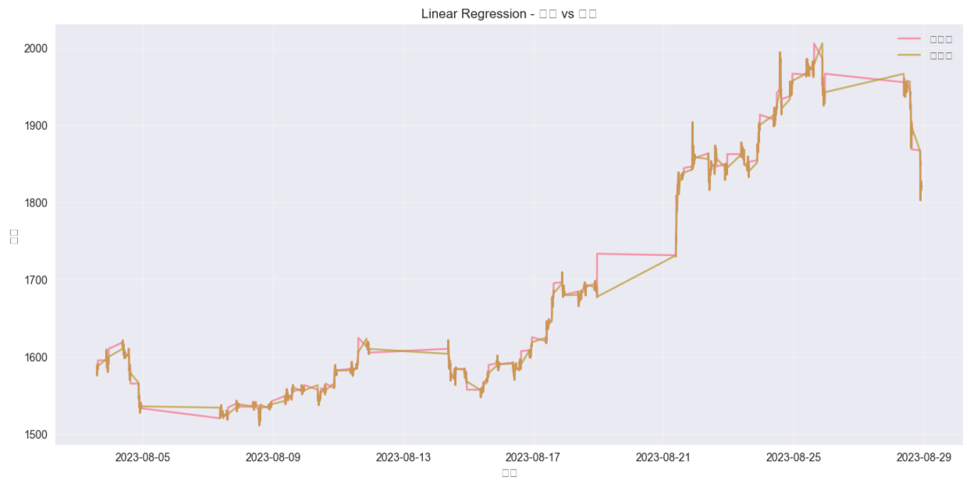
最佳模型预测结果可视化 1 2 3 4 5 6 7 8 9 10 11 12 13 14 15 16 17 18 19 20 21 22 23 24 25 26 27 28 29 30 best_model_name = results_df.index[0 ] print (f"最佳模型: {best_model_name} " )best_model = models[best_model_name] best_model.fit(X_train_scaled, y_train) y_pred = best_model.predict(X_test_scaled) plt.figure(figsize=(15 , 7 )) plt.plot(y_test.index, y_test.values, label='实际值' , alpha=0.7 ) plt.plot(y_test.index, y_pred, label='预测值' , alpha=0.7 ) plt.title(f'{best_model_name} - 预测 vs 实际' ) plt.xlabel('时间' ) plt.ylabel('价格' ) plt.legend() plt.grid(True , alpha=0.3 ) plt.show() residuals = y_test - y_pred plt.figure(figsize=(12 , 6 )) plt.scatter(y_pred, residuals, alpha=0.5 ) plt.axhline(y=0 , color='r' , linestyle='--' ) plt.title('残差图' ) plt.xlabel('预测值' ) plt.ylabel('残差' ) plt.grid(True , alpha=0.3 ) plt.show()
特征重要性分析(对于树模型) 1 2 3 4 5 6 7 8 9 10 11 12 13 14 15 16 17 18 19 20 21 22 23 24 25 26 27 28 29 if hasattr (best_model, 'feature_importances_' ): feature_importance = pd.DataFrame({ 'feature' : feature_columns, 'importance' : best_model.feature_importances_ }) feature_importance = feature_importance.sort_values('importance' , ascending=False ) plt.figure(figsize=(12 , 8 )) plt.barh(feature_importance['feature' ][:15 ], feature_importance['importance' ][:15 ]) plt.title('Top 15 特征重要性' ) plt.xlabel('重要性' ) plt.tight_layout() plt.show() elif hasattr (best_model, 'coef_' ): feature_importance = pd.DataFrame({ 'feature' : feature_columns, 'coefficient' : best_model.coef_ }) feature_importance = feature_importance.sort_values('coefficient' , key=abs , ascending=False ) plt.figure(figsize=(12 , 8 )) plt.barh(feature_importance['feature' ][:15 ], feature_importance['coefficient' ][:15 ]) plt.title('Top 15 特征系数(绝对值)' ) plt.xlabel('系数值' ) plt.tight_layout() plt.show()
时间序列交叉验证 1 2 3 4 5 6 7 8 9 10 11 12 13 14 15 16 17 18 19 20 21 22 23 24 25 26 27 28 29 tscv = TimeSeriesSplit(n_splits=5 ) model = GradientBoostingRegressor(n_estimators=100 , random_state=42 ) cv_scores = [] for train_index, test_index in tscv.split(X): X_train_cv, X_test_cv = X.iloc[train_index], X.iloc[test_index] y_train_cv, y_test_cv = y.iloc[train_index], y.iloc[test_index] X_train_cv_scaled = scaler.fit_transform(X_train_cv) X_test_cv_scaled = scaler.transform(X_test_cv) model.fit(X_train_cv_scaled, y_train_cv) y_pred_cv = model.predict(X_test_cv_scaled) score = r2_score(y_test_cv, y_pred_cv) cv_scores.append(score) print ("交叉验证R²分数:" , cv_scores)print ("平均R²分数:" , np.mean(cv_scores))print ("R²分数标准差:" , np.std(cv_scores))plt.figure(figsize=(10 , 6 )) plt.plot(range (1 , 6 ), cv_scores, marker='o' ) plt.title('时间序列交叉验证性能' ) plt.xlabel('折数' ) plt.ylabel('R²分数' ) plt.grid(True , alpha=0.3 ) plt.show()
当然还可以超参数调优,这里就不继续了
模型部署和预测 1 2 3 4 5 6 7 8 9 10 11 12 13 14 15 16 17 18 19 20 21 22 23 24 25 26 27 28 29 30 31 32 33 34 35 36 # 使用最佳模型进行未来预测 def predict_future_price(model, last_known_data, scaler, steps=1): """ 使用训练好的模型预测未来价格 参数: model: 训练好的模型 last_known_data: 最后已知的数据点(DataFrame) scaler: 用于标准化的scaler steps: 预测步数 返回: predictions: 预测值列表 """ predictions = [] current_data = last_known_data.copy() for _ in range(steps): # 标准化当前数据 current_data_scaled = scaler.transform(current_data) # 预测下一步 next_price = model.predict(current_data_scaled)[0] predictions.append(next_price) # 更新当前数据(这里需要根据实际情况调整) # 在实际应用中,需要更复杂的逻辑来更新特征 current_data.iloc[0, 3] = next_price # 更新close价格 return predictions # 示例:使用最后一行数据进行预测 last_known = X.iloc[[-1]].copy() future_predictions = predict_future_price(best_model, last_known, scaler, steps=5) print("未来5期预测价格:", future_predictions)
1 未来5期预测价格: [np.float64(1832.2961094333193), np.float64(1840.6007680672349), np.float64(1847.2991579272611), np.float64(1852.7019599802757), np.float64(1857.0597639651191)]
具体对不对,能不能用,自己去查吧,哈哈哈~
相关文章